Nov. 20, 2017 · 18 min read

In this article we will introduce the main concepts about of the convolutional neural networks (CNN) and its application in the image classification task. Before describe in detail the architecture of the CNNs, we will let's get acquainted with some definitions that will allow us to facilitate the understanding how the CNNs work.
When we refer to a CNN, it is implicit that we are referring a Deep Learning too. What is deep learning ? The deep learning, is a set of automatic learning algorithms that attempts to model high-level abstractions from data, using architectures composed of multiple non-linear transformations (see reference 1 , 23). Deep learning is part of a broader set of machine learning methods based on learning data representations. For example, in a task of image recognition, the image can be represented in many forms e.g. like a matrix of pixels or like a bytes vector. However, some representations let us make more easy the learning action for a particular interest task.
The goal of research in this area is to define which representations are better and how to create models capable of learning from these representations through multiple transformations, and thus obtain high performance in the tasks assigned to these models (see reference 2 ,3).
While it is true that there is not single definition of deep learning, several publications focus on different characteristics such as:
They use a cascade of levels (usually call layers) with non-linear processing units to extract and transform variables. Each layer uses the output of the previous layer as input. The algorithms can use supervised learning or unsupervised learning, and applications include data modeling and pattern recognition.
It is based on the learning of multiple levels of characteristics or representations of data. The higher level characteristics are derived from the lower level characteristics to form a hierarchical representation.
Learn multiple levels of representation that correspond to different levels of abstraction. These levels form a hierarchy of concepts.
All these ways that define the deep learning have in common follow aspects: multiple levels of none-linear processing (usually call layers); and supervised or unsupervised learning of feature representations in each level. The levels form a hierarchy of characteristics from a lower level of abstraction to a higher one.
The deep learning algorithms contrast with other learning algorithms by the number of transformations applied to the input data as it propagates from the first none-lineal transformation (input layer) until to the last none-lineal transformation (output layer). Each of these transformations includes parameters that can be trained as weights and thresholds (see references 2 , 3). However, there is not a standard rules for the number of transformations (or layers) that make an algorithm deep, but most researchers in the field believe that deep learning involves more than two intermediate transformations.
Commonly, the multiples none-linear transformation in deep learning are included as hidden layers of deep neural networks (see reference 4). These architectures have been applied in different fields such as computer vision, speech recognition, natural language processing, audio recognition, social network filtering, machine translation, bioinformatics and drug design (see reference 5), where they have produced results comparable to and in some cases superior (see reference 6) to human experts (see 7).
Once already the general aspect of deep learning have been discussed, we will now formally introduce CNNs.
Convolutional Neural Networks are a category of Neural Networks that have proven very effective in areas such as image recognition and classification. CNNs have been successful in identifying faces, objects and traffic signs apart from powering vision in robots and self driving cars.
CNNs, therefore, are an important tool for most machine learning researchers today. However, understanding CNNs and learning to use them for the first time can sometimes be an intimidating experience. The main aim purpose of this article is to develop an understanding of how Convolutional Neural Networks work on images.
if you are a newbie in neural network topics, We would recommend to read some tutorials on Multilayer Perceptrons before proceeding for a better understanding of how CNNs work.
In the lasl years several new architectures of convolutional neural networks (8,9) have been proposed. However, many of them, use the main concepts from the LeNet. LeNet was one of the very first convolutional neural networks which helped propel the field of Deep Learning. This pioneering work by Yann LeCun was named LeNet5 after many previous successful iterations since the year 1998 (see 10). At that time the LeNet architecture was used mainly for character recognition tasks such as reading zip codes, digits, etc.
Below, we will develop an intuitive description of how the LeNet architecture learns to recognize images works.

Figure 1: A simple ConvNet. Source 11
The Convolutional Neural Network in Figure 1 is similar in architecture to the original LeNet and classifies an input image into four categories: dog, cat, boat or bird (the original LeNet was used mainly for character recognition tasks). As observe from figure 1, the net receive a boat image as input, then the network correctly assigns the highest probability for boat (0.94) among all four categories.
For the recognition of the image, the network takes account four main operations:
These operations are the basic components of each convolutional neuronal network. Thus, understanding how the CNNS work, is an important step to developing a solid understanding about of them. We will try to understand the what there are behind each of these operations.
Essentially, every image can be represented as a matrix of pixel values.

Figure 2: Every image is a matrix of pixel values. Source 12
Channel is a conventional term used to refer to a certain component of an image. For example, an image from a standard digital camera will have three channels – red, green and blue – , thus, you can imagine those as three 2d-matrices stacked over each other (one for each color), each having pixel values in the range 0 to 255. These kind of objects (these three 2d-matrices) are called tensors in a mathematical context.
CNNs derive their name from the “convolution” operator. The primary purpose of Convolution in case of a CNNs is to extract features from the input image. Convolution preserves the spatial relationship between pixels by learning image features using small squares of input data. We will not go into the mathematical details of Convolution here, but will try to understand how it works over images.
As we discussed above, every image can be considered as a matrix of pixel values. Consider a 5 x 5 image whose pixel values are only 0 and 1 (note that for a gray scale image, pixel values range from 0 to 255, the green matrix below is a special case where pixel values are only 0 and 1):

Also, consider another 3 x 3 matrix as shown below:

Then, the Convolution of the 5 x 5 image and the 3 x 3 matrix can be computed as shown in the animation in Figure 5 below:
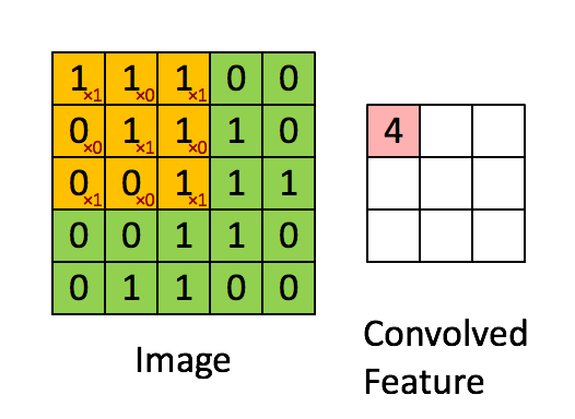
Figure 5: The Convolution operation. The output matrix is called Convolved Feature or Feature Map. Source 13
We take a moment to understand how the computation above is being done. We slide the orange matrix over our original image (green) by 1 pixel (also called ‘stride’) and for every position, we compute element wise multiplication (between the two matrices) and add the multiplication outputs to get the final integer which forms a single element of the output matrix (pink). Note that the 3×3 matrix “sees” only a part of the input image in each stride.
In CNNs terminology, the 3×3 matrix is called a ‘filter‘ or ‘kernel’ or ‘feature detector’ and the matrix formed by sliding the filter over the image and computing the dot product is called the ‘Convolved Feature’ or ‘Activation Map’ or the ‘Feature Map‘. It is important to note that filters acts as feature detectors from the original input image.
It is evident from the animation above that different values of the filter matrix will produce different Feature Maps for the same input image. As an example, consider the follow input image:

In the table below, we can see the effects of convolution of the above image with different filters. As shown, we can perform operations such as Edge Detection, Sharpen and Blur just by changing the numeric values of our filter matrix before the convolution operation (for more details see reference 14) – this means that different filters can detect different features from an image, for example edges, curves etc.
 Another example that illustrate the Convolution operation is by looking at the animation in Figure 8 below:
Figure 8: The Convolution Operation. Source 15
A filter (with red outline) slides over the input image (convolution operation) to produce a feature map. The convolution of another filter (with the green outline), over the same image gives a different feature map as shown. It is important to note that the Convolution operation captures the local dependencies in the original image. Also note how these two different filters generate different feature maps from the same original image. Remember that the image and the two filters above are just numeric matrices as we have discussed above.
In practice, a CNN learns the values of these filters on its own during the training process (although we still need to specify parameters such as number of filters, filter size, architecture of the network etc. before the training process). The more number of filters we have, the more image features get extracted and the better our network becomes at recognizing patterns in unseen images.
The size of the Feature Map (Convolved Feature) is controlled by three parameters 16 that we need to decide before the convolution step is performed:
Depth: Depth corresponds to the number of filters we use for the convolution operation (multiples none- linear transformation discussed above). In the network shown in Figure 9, we are performing convolution of the original boat image using three distinct filters, thus producing three different feature maps as shown. You can think of these three feature maps as stacked 2d matrices, so, the ‘depth’ of the feature map would be three.
Stride: Stride is the number of pixels by which we slide our filter matrix over the input matrix. When the stride is 1 then we move the filters one pixel at a time. When the stride is 2, then the filters jump 2 pixels at a time as we slide them around. Having a larger stride will produce smaller feature maps.
Zero-padding: Sometimes, it is convenient to pad the input matrix with zeros around the border, so that we can apply the filter to bordering elements of our input image matrix. A nice feature of zero padding is that it allows us to control the size of the feature maps. Adding zero-padding is also called wide convolution, and not using zero-padding would be a narrow convolution. This has been explained clearly in 17.
 Figure 9
An additional operation called ReLU has been used after every Convolution operation in Figure 10 above. ReLU stands for Rectified Linear Unit and is a non-linear operation. Its output is given by:
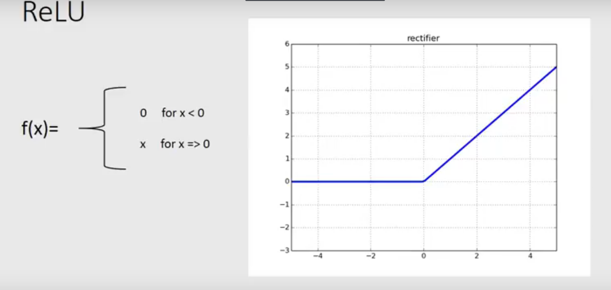 Figure 10: the ReLU operation
ReLU is an element wise operation (applied per pixel) and replace all negative pixel values in the feature map by zero.
The ReLU operation can be understood clearly from Figure 11 below. It shows the ReLU operation applied to one of the feature maps obtained in Figure 6 above. The output feature map here is also referred to as the ‘Rectified’ feature map.
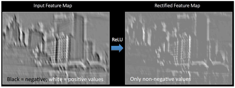 Figure 11 ReLu operation (see 18)
Spatial Pooling (also called sub-sampling or down-sampling) reduces the dimensionality of each feature map but retains the most important information. Spatial Pooling can be of different types: Max, Average, Sum etc.
In case of Max Pooling, we define a spatial neighborhood (for example, a 2×2 window) and take the largest element from the rectified feature map within that window. Instead of taking the largest element we could also take the average (Average Pooling) or sum of all elements in that window. In practice, Max Pooling has been shown to work better.
Figure 12 shows an example of Max Pooling operation on a Rectified Feature map (obtained after convolution + ReLU operation) by using a 2×2 window.
 Figure 12: Max Pooling Operation. (Rectified Feature Map). 16
We slide our 2 x 2 window by 2 cells (also called ‘stride’) and take the maximum value in each region. As shown in Figure 10, this reduces the dimensionality of our feature map.
In the network shown in Figure 13, pooling operation is applied separately to each feature map (notice that, due to this, we get three output maps from three input maps).
 Figure 13: Pooling applied to Rectified Feature Maps
Figure 14 shows the effect of Pooling on the Rectified Feature Map we received after the ReLU operation in Figure 11 above.
 Figure 14: Pooling. Source 18
The function of Pooling is to progressively reduce the spatial size of the input representation 16. In particular, pooling
makes the input representations (feature dimension) smaller and more manageable
reduces the number of parameters and computations in the network, therefore, controlling overfitting 16
makes the network invariant to small transformations, distortions and translations in the input image (a small distortion in input will not change the output of Pooling – since we take the maximum / average value in a local neighborhood).
helps us arrive at an almost scale invariant representation of our image (the exact term is “equivariant”). This is very powerful since we can detect objects in an image no matter where they are located (read 18 for details).
So far we have seen how the Convolution, ReLU and Pooling layers work. It is important to understand that these layers are the basic building blocks of any CNN. As shown in Figure 15, we have two sets of Convolution, ReLU & Pooling layers – the 2nd Convolution layer performs convolution on the output of the first Pooling Layer using six filters to produce a total of six feature maps. ReLU is then applied individually on all of these six feature maps. We then perform Max Pooling operation separately on each of the six rectified feature maps.
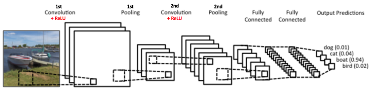 Figure 15
Together these layers extract the useful features from the images, introduce non-linearity in our network and reduce feature dimension while aiming to make the features somewhat equivariant to scale and translation 19.
The output of the 2nd Pooling Layer acts as an input to the Fully Connected Layer, which we will discuss in the next part.
The Fully Connected layer is a traditional Multi Layer Perceptron (20) that uses a softmax activation function in the output layer (other classifiers like SVM can also be used, but will stick to softmax in this post). The term “Fully Connected” implies that every neuron in the previous layer is connected to every neuron on the next layer.
The output from the convolutional and pooling layers represent high-level features of the input image. The purpose of the Fully Connected layer is to use these features for classifying the input image into various classes based on the training dataset. For example, the image classification task we set out to perform has four possible outputs as shown in Figure 14 below (note that Figure 14 does not show connections between the nodes in the fully connected layer).
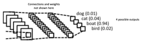 Figure 16: Fully Connected Layer -each node is connected to every other node in the adjacent layer
Adding a fully-connected layer is a cheap way of learning non-linear combinations of features obtained trrought of the convolution processes. Most of the features from convolutional and pooling layers may be good for the classification task, but combinations of those features might be even better.
The sum of output probabilities from the Fully Connected Layer is 1. This is ensured by using the Softmax as the activation function in the output layer of the Fully Connected Layer. The Softmax function takes a vector of arbitrary real-valued scores and squashes it to a vector of values between zero and one that sum to one.
Combining all processes above explained, where the Convolution + Pooling layers act as Feature Extractors from the input image; while Fully Connected layer acts as a classifier.
Thus, going back to the initial example in which we want to classify the input image (see Figure 16 showed below).
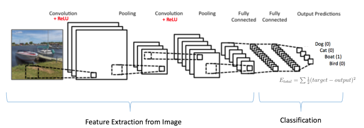 Figure 17: Training the ConvNet
Since the input image is a boat, the target probability is 1 for Boat class and 0 for other three classes, i.e.
Input Image = Boat
Output: Target vector [0,0,1,0] ([prob. to be Dog, prob to be cat, prob to be Boat, prob to be Bird])
In addition to the architecture of the neural network, another important aspect is the optimization of all its parameters. This implies the values of the thresholds for the filters that we have to choose, as well as, the weights of the connections in the layers of the multiperceptrons. The optimization process of all these parameters is defined as the training process of the network.
The overall training process of the Convolution Network may be summarized as below:
The above steps train the ConvNet – this essentially means that all the weights and parameters of the ConvNet have now been optimized to correctly classify images from the training set.
When a new (unseen) image is input into the ConvNet, the network would go through the forward propagation step and output a probability for each class (for a new image, the output probabilities are calculated using the weights which have been optimized to correctly classify all the previous training examples). If our training set is large enough, the network will (hopefully) generalize well to new images and classify them into correct categories.
The steps above have been oversimplified and mathematical details have been avoided to provide intuition into the training process. See 16 for a mathematical formulation and thorough understanding.
In the example above we used two sets of alternating Convolution and Pooling layers. Please note however, that these operations can be repeated any number of times in a single ConvNet. In fact, some of the best performing ConvNets today have tens of Convolution and Pooling layers! Also, it is not necessary to have a Pooling layer after every Convolutional Layer.
Convolutional Neural Networks have been used since early 1990s. We discussed the LeNet above which was one of the very first convolutional neural networks in order to the readers have intuitions about how the CNNs work. Some other influential architectures are listed below
LeNet (1990s): Already covered in this article.
1990s to 2012: In the years from late 1990s to early 2010s convolutional neural network were in incubation. As more and more data and computing power became available, tasks that convolutional neural networks could tackle became more and more interesting.
AlexNet (2012) – In 2012, Alex Krizhevsky (and others) released AlexNet which was a deeper and much wider version of the LeNet and won by a large margin the difficult ImageNet Large Scale Visual Recognition Challenge (ILSVRC) in 2012. It was a significant breakthrough with respect to the previous approaches and the current widespread application of CNNs can be attributed to this work.
ZF Net (2013) – The ILSVRC 2013 winner was a Convolutional Network from Matthew Zeiler and Rob Fergus. It became known as the ZFNet (short for Zeiler & Fergus Net). It was an improvement on AlexNet by tweaking the architecture hyperparameters.
GoogLeNet (2014) – The ILSVRC 2014 winner was a Convolutional Network from Szegedy et al. from Google. Its main contribution was the development of an Inception Module that dramatically reduced the number of parameters in the network (4M, compared to AlexNet with 60M).
VGGNet (2014) – The runner-up in ILSVRC 2014 was the network that became known as the VGGNet. Its main contribution was in showing that the depth of the network (number of layers) is a critical component for good performance.
ResNets (2015) – Residual Network developed by Kaiming He (and others) was the winner of ILSVRC 2015. ResNets are currently by far state of the art Convolutional Neural Network models and are the default choice for using ConvNets in practice (as of May 2016).
DenseNet (August 2016) – Recently published by Gao Huang (and others), the Densely Connected Convolutional Network has each layer directly connected to every other layer in a feed-forward fashion. The DenseNet has been shown to obtain significant improvements over previous state-of-the-art architectures on five highly competitive object recognition benchmark tasks. Check out the Torch implementation here.
In this article, we have explained the main concepts behind Convolutional Neural Networks in simple terms. There are several details that we have oversimplified / skipped, but hopefully this post gave you some intuition around how they work.
All images and animations used in this post belong to their respective authors as listed in References section below.
1 Y. Bengio, A. Courville, and P. Vincent., "Representation Learning: A Review and New Perspectives," IEEE Trans. PAMI, special issue Learning Deep Architectures, 2013
2 JürgenSchmidhuber., Neural Networks Volume 61, January 2015, Pages 85-117
3 Deng, L.; Yu, D. (2014). "Deep Learning: Methods and Applications" (PDF). Foundations and Trends in Signal Processing. 7 (3–4): 1–199. doi:10.1561/2000000039
4 Bengio, Yoshua (2009). "Learning Deep Architectures for AI" (PDF). Foundations and Trends in Machine Learning. 2 (1): 1–127. doi:10.1561/2200000006.
5 Ghasemi, F.; Mehridehnavi, AR.; Fassihi, A.; Perez-Sanchez, H. (2017). "Deep Neural Network in Biological Activity Prediction using Deep Belief Network". Applied Soft Computing.
6 Ciresan, Dan; Meier, U.; Schmidhuber, J. (June 2012). "Multi-column deep neural networks for image classification". 2012 IEEE Conference on Computer Vision and Pattern Recognition: 3642–3649. doi:10.1109/cvpr.2012.6248110.
7 Krizhevsky, Alex; Sutskever, Ilya; Hinton, Geoffry (2012). "ImageNet Classification with Deep Convolutional Neural Networks". NIPS 2012: Neural Information Processing Systems, Lake Tahoe, Nevada.
8 LeCun, Yann; Bottou Léon; Bengio Yoshua and Haffiner Patric. (1998). "Gradient-Based Learning Applied to Document Recognition". Proc. of the IEE.
11 Clarifai / Technology
12 Machine Learning is Fun! Part 3: Deep Learning and Convolutional Neural Networks
13 Feature extraction using convolution, Stanford
14 Wikipedia article on Kernel (image processing)
15 Deep Learning Methods for Vision, CVPR 2012 Tutorial
16 CS231n Convolutional Neural Networks for Visual Recognition, Stanford
17 Understanding Convolutional Neural Networks for NLP
18 Neural Networks by Rob Fergus, Machine Learning Summer School 2015
19 What is the difference between deep learning and usual machine learning?
20 Introduction to Multi-Layer Perceptrons
21 How the backpropagation algorithm works
22 Artificial Neural Networks: Mathematics of Backpropagation
23 Deep Learning with Neural Networks and TensorFlow Introduction


