10 de Enero de 2018 · 15 min de lectura

En el tutorial anterior (Tutorial II) se mostró cómo implementar una red neuronal convolucional en TensorFlow. En dicho tutorial, se requería un conocimiento a bajo nivel de cómo funciona TensorFlow para el diseño e implementación de la red neuronal.
En éste tutorial, y para el mismo ejemplo práctico usado en el Tutorial II (reconocimiento de dígitos escritos a mano), vamos explicar como usar el paquete adicional para TensorFlow llamado PrettyTensor, también desarrollado por Google, para crear la arquitectura de la red convolucional empleada en el Tutorial II. PrettyTensor proporciona formas mucho más simples de construir redes neuronales en TensorFlow, lo que nos permite centrarnos en la arquitectura de la red que a construir y no preocuparnos demasiado por los detalles de implementación a bajo nivel. Esto hace que el código fuente sea mucho más corto, fácil de leer y modificar.
La mayor parte del código fuente en este tutorial es idéntico al Tutorial II, excepto por la construcción de los grafos, que ahora se hace usando PrettyTensor, así como algunos cambios menores que idicaremos en el desarrollo de éste artículo, por lo que recomendamos revisar nuestro Tutorial II.
Antes de continuar, recordemos el esquema de la red neuronal convolucinal que queremos implementar para la tarea del reconocimiento de dígitos escritos a mano, para ello veamos la siguinete imagen ya empleada en el Tutorial II.

Comenzamos por importar algunas librerias, incluyendo la librería PrettyTensor
%matplotlib inline
import matplotlib.pyplot as plt
import tensorflow as tf
import numpy as np
from sklearn.metrics import confusion_matrix
import time
from datetime import timedelta
import math

# We also need PrettyTensor.
import prettytensor as pt
Cargamos el conjunto de datos MNIST que se descargará automáticamente si no se encuentra en la ruta dada.
from tensorflow.examples.tutorials.mnist import input_data
data = input_data.read_data_sets('data/MNIST/', one_hot=True)
Extracting data/MNIST/train-images-idx3-ubyte.gz
Extracting data/MNIST/train-labels-idx1-ubyte.gz
Extracting data/MNIST/t10k-images-idx3-ubyte.gz
Extracting data/MNIST/t10k-labels-idx1-ubyte.gz
Verificamos los datos
print("Size of:")
print("- Training-set:\t\t{}".format(len(data.train.labels)))
print("- Test-set:\t\t{}".format(len(data.test.labels)))
print("- Validation-set:\t{}".format(len(data.validation.labels)))
Size of:
Training-set: 55000
Test-set: 10000
Validation-set: 5000
Como se observa, ahora tenemos tres sub conjunto de datos, uno de entrenamiento, uno de test y otro de validación.
El conjunto de datos se ha cargado con la codificación denominada One-Hot. Esto significa que las etiquetas se han convertido de un solo número a un vector cuya longitud es igual a la cantidad de clases posibles. Todos los elementos del vector son cero excepto el elemento i enésimo que toma el valor uno; y significa que la clase es i.
Por ejemplo, las etiquetas codificadas de One-Hot para las primeras 5 imágenes en el conjunto de prueba son:
data.test.labels[0:5, :]
se obtiene:
  array([[ 0.,  0.,  0.,  0.,  0.,  0.,  0.,  1.,  0.,  0.],
         [ 0.,  0.,  1.,  0.,  0.,  0.,  0.,  0.,  0.,  0.],
         [ 0.,  1.,  0.,  0.,  0.,  0.,  0.,  0.,  0.,  0.],
         [ 1.,  0.,  0.,  0.,  0.,  0.,  0.,  0.,  0.,  0.],
         [ 0.,  0.,  0.,  0.,  1.,  0.,  0.,  0.,  0.,  0.]])
Como se observa, tenemos cinco vectores donde cada componete tiene valores cero excepto en la posición de la componete que identifica la clase, cuyo valor es 1.
Como necesitamos las clases como números únicos para las comparaciones y medidas de rendimiento, procedemos a convertir estos vectores codificados como One-Hot a un solo número tomando el índice del elemento más alto. Tenga en cuenta que la palabra 'clase' es una palabra clave utilizada en Python, por lo que necesitamos usar el nombre 'cls' en su lugar.
Para codificar estos vectores a números:
data.test.cls = np.argmax(data.test.labels, axis=1)
Ahora podemos ver la clase para las primeras cinco imágenes en el conjunto de pruebas.
print (data.test.cls[0:5])
se obtiene
array([7, 2, 1, 0, 4, 1])
Comparemos estos con los vectores codificados One-Hot de arriba. Por ejemplo, la clase para la primera imagen es 7, que corresponde a un vector codificado One-Hot donde todos los elementos son cero excepto el elemento con índice 7.
Pasamos a definir el conjunto de variables para dar formato a las dimensiones de nuestras imágenes:
# We know that MNIST images are 28 pixels in each dimension.
img_size = 28

# Images are stored in one-dimensional arrays of this length.
img_size_flat = img_size * img_size

# Tuple with height and width of images used to reshape arrays.
img_shape = (img_size, img_size)

# Number of colour channels for the images: 1 channel for gray-scale.
num_channels = 1

# Number of classes, one class for each of 10 digits.
num_classes = 10
Ahora crearemos una función que es utilizada para trazar 9 imágenes en una cuadrícula de 3x3 y escribir las clases verdaderas y predichas debajo de cada imagen.
def plot_images(images, cls_true, cls_pred=None):
    assert len(images) == len(cls_true) == 9

    # Create figure with 3x3 sub-plots.
    fig, axes = plt.subplots(3, 3)
    fig.subplots_adjust(hspace=0.3, wspace=0.3)

    for i, ax in enumerate(axes.flat):
        # Plot image.
        ax.imshow(images[i].reshape(img_shape), cmap='binary')

        # Show true and predicted classes.
        if cls_pred is None:
            xlabel = "True: {0}".format(cls_true[i])
        else:
            xlabel = "True: {0}, Pred: {1}".format(cls_true[i], cls_pred[i])

        # Show the classes as the label on the x-axis.
        ax.set_xlabel(xlabel)

        # Remove ticks from the plot.
        ax.set_xticks([])
        ax.set_yticks([])

    # Ensure the plot is shown correctly with multiple plots
    # in a single Notebook cell.
    plt.show()
Graficamos algunas imágenes para ver si los datos son correctos
# Get the first images from the test-set.
images = data.test.images[0:9]

# Get the true classes for those images.
cls_true = data.test.cls[0:9]

# Plot the images and labels using our helper-function above.
plot_images(images=images, cls_true=cls_true)

Creamos las variables de marcador de posición como se ha hecho en el Tutorial II
x = tf.placeholder(tf.float32, shape=[None, img_size_flat], name='x')
x_image = tf.reshape(x, [-1, img_size, img_size, num_channels])
y_true = tf.placeholder(tf.float32, shape=[None, num_classes], name='y_true')
y_true_cls = tf.argmax(y_true, dimension=1)
Esta sección muestra cómo realizar exactamente la misma implementación de la red neuronal convolucional en el Tutorial II utilizando PrettyTensor.
La idea básica es transformar el tensor de entrada x_image en un objeto PrettyTensor que tiene funciones auxiliares para agregar nuevas capas computacionales a fin de crear una Red Neural completa. Esto es un poco similar a las funciones auxiliares que implementamos anteriormente, pero es aún más simple porque PrettyTensor también realiza un seguimiento de las dimensiones de entrada y salida de cada capa.
x_pretty = pt.wrap(x_image)
Ahora que hemos transformado la imagen de entrada en un objeto PrettyTensor, podemos agregar, tanto las capas convolucionales, como las capas totalmente conectadas en unas pocas líneas de código fuente.
with pt.defaults_scope(activation_fn=tf.nn.relu):
    y_pred, loss = x_pretty.\
        conv2d(kernel=5, depth=16, name='layer_conv1').\
        max_pool(kernel=2, stride=2).\
        conv2d(kernel=5, depth=36, name='layer_conv2').\
        max_pool(kernel=2, stride=2).\
        flatten().\
        fully_connected(size=128, name='layer_fc1').\
        softmax_classifier(num_classes=num_classes, labels=y_true)
Tenga en cuenta que en la función pt.defaults_scope (activation_fn = tf.nn.relu) , introduce la función de activiación activation_fn = tf.nn.relu como argumento para cada una de las capas construidas dentro del bloque with , de modo que las unidades lineales rectificadas (ReLU) se usan para cada uno de estas capas. El * defaults_scope * hace que sea fácil cambiar los argumentos para todas las capas.
¡Eso es! Ahora hemos creado exactamente la misma red neuronal convolucional implementada en el Tutorial II en unas simples líneas de código, en contraste a las numerosas líneas de código que se requerían muchas en la implementación directa con TensorFlow.
Usando PrettyTensor, podemos ver claramente la estructura de la red y cómo los datos fluyen a través de la red. Esto nos permite centrarnos en las ideas principales de la Red Neural en lugar de detalles de implementación a bajo nivel. ¡Es simple y bonito!
Lamentablemente, no todo es tan directo cuando se usa PrettyTensor.
Por ejemplo, si más adelante, queremos trazar los pesos de las capas convolucionales, la forma de recuperar estos pesos no es tan directa. En la implementación de TensorFlow (ver Tutorial II), nosotros mismos habíamos creado las variables, por lo que pudimos referirnos directamente a ellas. Pero cuando la red se construye utilizando PrettyTensor, todas las variables de las capas se crean indirectamente mediante PrettyTensor. Por lo tanto, tenemos que recuperar las variables de TensorFlow.
Para ello utilizamos los nombres layer_conv1 y layer_conv2 para las dos capas convolucionales. Estos también se denominan variable scopes (no deben confundirse con defaults_scope). PrettyTensor asigna automáticamente nombres a las variables que crea para cada capa, de modo que podemos recuperar los pesos de una capa usando el nombre de la variable scopes de la capa y el nombre de la variable.
La implementación es algo incómoda porque tenemos que usar la función TensorFlow get_variable () que fue diseñada para otro propósito; ya sea creando una nueva variable o reutilizando una variable existente. Lo más fácil es hacer la siguiente función auxiliar.
def get_weights_variable(layer_name):
    # Retrieve an existing variable named 'weights' in the scope
    # with the given layer_name.
    # This is awkward because the TensorFlow function was
    # really intended for another purpose.

    with tf.variable_scope(layer_name, reuse=True):
        variable = tf.get_variable('weights')

    return variable
Usando esta función podemos recuperar las variables como objetos TensorFlow. Para obtener los contenidos de las variables, debe hacer algo como: contents = session.run(weights_conv1) como se muestrará más adelante.
Obtenemos los pesos:
weights_conv1 = get_weights_variable(layer_name='layer_conv1')
weights_conv2 = get_weights_variable(layer_name='layer_conv2')
PrettyTensor nos devuelve la etiqueta de clase class-label (y_pred) , así como una medida de pérdida que debe minimizarse, para mejorar la capacidad de la Red Neural para clasificar las imágenes de entrada.
Tenga en cuenta que la optimización no se realiza en este momento. De hecho, nada se calcula en absoluto, simplemente agregamos el objeto optimizador (optimizer-object) al grafo TensorFlow para su posterior ejecución.
optimizer = tf.train.AdamOptimizer(learning_rate=1e-4).minimize(loss)
Necesitamos algunas medidas de rendimiento más para mostrar el progreso al usuario.
Primero calculamos el número de clase predicho a partir de la salida de la Red Neural y_pred , que es un vector con 10 elementos. El número de clase es el índice del elemento más grande.
y_pred_cls = tf.argmax(y_pred, dimension=1)
Luego creamos un vector de booleanos que nos dice si la clase predicha es igual a la clase verdadera de cada imagen.
correct_prediction = tf.equal(y_pred_cls, y_true_cls)
Calculamos la precisión (accuracy) de la clasificación y transforma los booleanos a floats, de modo que False se convierte en 0 y True se convierte en 1. Luego calculamos el promedio de estos números.
accuracy = tf.reduce_mean(tf.cast(correct_prediction, tf.float32))
Una vez que se ha creado la red, tenemos que crear una sesión de TensorFlow y ejecutar el grafo.
session = tf.Session()
Inicializamos las variables:
session.run(tf.global_variables_initializer())
creamos la función de iteración para el proceso de optimización:
train_batch_size = 64

# Counter for total number of iterations performed so far.
total_iterations = 0

def optimize(num_iterations):
    # Ensure we update the global variable rather than a local copy.
    global total_iterations

    # Start-time used for printing time-usage below.
    start_time = time.time()

    for i in range(total_iterations,
                   total_iterations + num_iterations):

        # Get a batch of training examples.
        # x_batch now holds a batch of images and
        # y_true_batch are the true labels for those images.
        x_batch, y_true_batch = data.train.next_batch(train_batch_size)

        # Put the batch into a dict with the proper names
        # for placeholder variables in the TensorFlow graph.
        feed_dict_train = {x: x_batch,
                           y_true: y_true_batch}

        # Run the optimizer using this batch of training data.
        # TensorFlow assigns the variables in feed_dict_train
        # to the placeholder variables and then runs the optimizer.
        session.run(optimizer, feed_dict=feed_dict_train)

        # Print status every 100 iterations.
        if i % 100 == 0:
            # Calculate the accuracy on the training-set.
            acc = session.run(accuracy, feed_dict=feed_dict_train)

            # Message for printing.
            msg = "Optimization Iteration: {0:>6}, Training Accuracy: {1:>6.1%}"

            # Print it.
            print(msg.format(i + 1, acc))

    # Update the total number of iterations performed.
    total_iterations += num_iterations

    # Ending time.
    end_time = time.time()

    # Difference between start and end-times.
    time_dif = end_time - start_time

    # Print the time-usage.
    print("Time usage: " + str(timedelta(seconds=int(round(time_dif)))))
Ahora crearemos algunas funciones para el monitoreo del comportamiento del modelo.
def plot_example_errors(cls_pred, correct):
    # This function is called from print_test_accuracy() below.

    # cls_pred is an array of the predicted class-number for
    # all images in the test-set.

    # correct is a boolean array whether the predicted class
    # is equal to the true class for each image in the test-set.

    # Negate the boolean array.
    incorrect = (correct == False)

    # Get the images from the test-set that have been
    # incorrectly classified.
    images = data.test.images[incorrect]

    # Get the predicted classes for those images.
    cls_pred = cls_pred[incorrect]

    # Get the true classes for those images.
    cls_true = data.test.cls[incorrect]

    # Plot the first 9 images.
    plot_images(images=images[0:9],
                cls_true=cls_true[0:9],
                cls_pred=cls_pred[0:9])
def plot_confusion_matrix(cls_pred):
    # This is called from print_test_accuracy() below.

    # cls_pred is an array of the predicted class-number for
    # all images in the test-set.

    # Get the true classifications for the test-set.
    cls_true = data.test.cls

    # Get the confusion matrix using sklearn.
    cm = confusion_matrix(y_true=cls_true,
                          y_pred=cls_pred)

    # Print the confusion matrix as text.
    print(cm)

    # Plot the confusion matrix as an image.
    plt.matshow(cm)

    # Make various adjustments to the plot.
    plt.colorbar()
    tick_marks = np.arange(num_classes)
    plt.xticks(tick_marks, range(num_classes))
    plt.yticks(tick_marks, range(num_classes))
    plt.xlabel('Predicted')
    plt.ylabel('True')

    # Ensure the plot is shown correctly with multiple plots
    # in a single Notebook cell.
    plt.show()
# Split the test-set into smaller batches of this size.
test_batch_size = 256

def print_test_accuracy(show_example_errors=False,
                        show_confusion_matrix=False):

    # Number of images in the test-set.
    num_test = len(data.test.images)

    # Allocate an array for the predicted classes which
    # will be calculated in batches and filled into this array.
    cls_pred = np.zeros(shape=num_test, dtype=np.int)

    # Now calculate the predicted classes for the batches.
    # We will just iterate through all the batches.
    # There might be a more clever and Pythonic way of doing this.

    # The starting index for the next batch is denoted i.
    i = 0

    while i < num_test:
        # The ending index for the next batch is denoted j.
        j = min(i + test_batch_size, num_test)

        # Get the images from the test-set between index i and j.
        images = data.test.images[i:j, :]

        # Get the associated labels.
        labels = data.test.labels[i:j, :]

        # Create a feed-dict with these images and labels.
        feed_dict = {x: images,
                     y_true: labels}

        # Calculate the predicted class using TensorFlow.
        cls_pred[i:j] = session.run(y_pred_cls, feed_dict=feed_dict)

        # Set the start-index for the next batch to the
        # end-index of the current batch.
        i = j

    # Convenience variable for the true class-numbers of the test-set.
    cls_true = data.test.cls

    # Create a boolean array whether each image is correctly classified.
    correct = (cls_true == cls_pred)

    # Calculate the number of correctly classified images.
    # When summing a boolean array, False means 0 and True means 1.
    correct_sum = correct.sum()

    # Classification accuracy is the number of correctly classified
    # images divided by the total number of images in the test-set.
    acc = float(correct_sum) / num_test

    # Print the accuracy.
    msg = "Accuracy on Test-Set: {0:.1%} ({1} / {2})"
    print(msg.format(acc, correct_sum, num_test))

    # Plot some examples of mis-classifications, if desired.
    if show_example_errors:
        print("Example errors:")
        plot_example_errors(cls_pred=cls_pred, correct=correct)

    # Plot the confusion matrix, if desired.
    if show_confusion_matrix:
        print("Confusion Matrix:")
        plot_confusion_matrix(cls_pred=cls_pred)
Miremos la precisión antes de cualquier optimización.
print_test_accuracy()
Accuracy on Test-Set: 11.4% (1139 / 10000)
Como vemos, la precisión del modelo es muy baja. Tiene sentido, puesto que no hemos optimizado ningún parámetro.
Mirémos ahora depuès de una iteración en el proceso de optimización:
optimize(num_iterations=1)
Optimization Iteration: 1, Training Accuracy: 10.9%
Time usage: 0:00:00
print_test_accuracy()
Accuracy on Test-Set: 13.1% (1309 / 10000)
como vemos como el modelo mejora un poco su precisión.
Rendimiento después de 100 iteraciones de optimización
optimize(num_iterations=99) # We already performed 1 iteration above.
Time usage: 0:00:08
print_test_accuracy(show_example_errors=False)
Accuracy on Test-Set: 84.3% (8432 / 10000)
Después de 100 iteraciones de optimización, el modelo ha mejorado significativamente su precisión de clasificación.
Rendimiento después de 1000 iteraciones de optimización
optimize(num_iterations=900) # We performed 100 iterations above.
Optimization Iteration: 101, Training Accuracy: 87.5%
Optimization Iteration: 201, Training Accuracy: 87.5%
Optimization Iteration: 301, Training Accuracy: 84.4%
Optimization Iteration: 401, Training Accuracy: 85.9%
Optimization Iteration: 501, Training Accuracy: 89.1%
Optimization Iteration: 601, Training Accuracy: 95.3%
Optimization Iteration: 701, Training Accuracy: 96.9%
Optimization Iteration: 801, Training Accuracy: 93.8%
Optimization Iteration: 901, Training Accuracy: 98.4%
Time usage: 0:01:14
print_test_accuracy(show_example_errors=False)
Después de 10.000 iteraciones
optimize(num_iterations=9000) # We performed 1000 iterations above.
Optimization Iteration: 8601, Training Accuracy: 100.0%
Optimization Iteration: 8701, Training Accuracy: 100.0%
Optimization Iteration: 8801, Training Accuracy: 100.0%
Optimization Iteration: 8901, Training Accuracy: 100.0%
Optimization Iteration: 9001, Training Accuracy: 98.4%
Optimization Iteration: 9101, Training Accuracy: 100.0%
Optimization Iteration: 9201, Training Accuracy: 100.0%
Optimization Iteration: 9301, Training Accuracy: 96.9%
Optimization Iteration: 9401, Training Accuracy: 100.0%
Optimization Iteration: 9501, Training Accuracy: 100.0%
Optimization Iteration: 9601, Training Accuracy: 100.0%
Optimization Iteration: 9701, Training Accuracy: 100.0%
Optimization Iteration: 9801, Training Accuracy: 100.0%
Optimization Iteration: 9901, Training Accuracy: 100.0%
Time usage: 0:12:50
print_test_accuracy(show_example_errors=False,
                    show_confusion_matrix=True)
Accuracy on Test-Set: 98.9% (9889 / 10000)
Confusion Matrix:
[[ 973    0    0    0    0    1    2    1    3    0]
 [   0 1133    1    0    0    0    0    0    1    0]
 [   2    2 1015    2    1    0    1    3    6    0]
 [   0    0    0 1007    0    1    0    0    2    0]
 [   0    0    0    0  978    0    0    0    0    4]
 [   2    0    1    6    0  876    1    0    3    3]
 [   7    3    0    1    1    1  945    0    0    0]
 [   0    2    7    2    1    0    0 1006    1    9]
 [   4    0    2    0    1    1    0    2  961    3]
 [   0    3    0    1    5    4    0    0    1  995]]

Cuando la red neuronal convolucional se implementó directamente en TensorFlow, podemos graficar fácilmente tanto los pesos convolucionales como las imágenes que salieron de las diferentes capas. Sin embargo, cuando se emplea PrettyTensor recuperar los pesos y las imágenes no es tan directo, pero podemos recuperar las imágenes que salen de las capas convolucionales, creamos una función para ello:
def plot_conv_weights(weights, input_channel=0):
    # Assume weights are TensorFlow ops for 4-dim variables
    # e.g. weights_conv1 or weights_conv2.

    # Retrieve the values of the weight-variables from TensorFlow.
    # A feed-dict is not necessary because nothing is calculated.
    w = session.run(weights)

    # Get the lowest and highest values for the weights.
    # This is used to correct the colour intensity across
    # the images so they can be compared with each other.
    w_min = np.min(w)
    w_max = np.max(w)

    # Number of filters used in the conv. layer.
    num_filters = w.shape[3]

    # Number of grids to plot.
    # Rounded-up, square-root of the number of filters.
    num_grids = math.ceil(math.sqrt(num_filters))

    # Create figure with a grid of sub-plots.
    fig, axes = plt.subplots(num_grids, num_grids)

    # Plot all the filter-weights.
    for i, ax in enumerate(axes.flat):
        # Only plot the valid filter-weights.
        if i<num_filters:
            # Get the weights for the i'th filter of the input channel.
            # See new_conv_layer() for details on the format
            # of this 4-dim tensor.
            img = w[:, :, input_channel, i]

            # Plot image.
            ax.imshow(img, vmin=w_min, vmax=w_max,
                      interpolation='nearest', cmap='seismic')

        # Remove ticks from the plot.
        ax.set_xticks([])
        ax.set_yticks([])

    # Ensure the plot is shown correctly with multiple plots
    # in a single Notebook cell.
    plt.show()
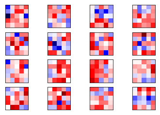
Ahora mostramos los imágenes de los pesos de los filtros en la primera capa de convolución de la red (rojo para valores positivos y azules para valores negativos):
plot_conv_weights(weights=weights_conv1)
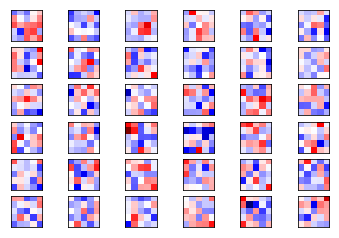
Ahora grafica los pesos de los filtros para la segunda capa convolucional. Dado que hay 16 canales de salida desde la primera capa convolucional, entonces tendremos 16 canales de entrada para la segunda capa convolucional. La segunda capa convolucional tiene un conjunto de filtros de los pesos para cada uno de sus canales de entrada. Comenzamos por graficar los pesos del filtro para el primer canal. Note nuevamente que los pesos positivos son rojos y los pesos negativos son azules.
plot_conv_weights(weights=weights_conv2, input_channel=0)
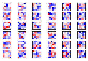
Ahora para el canal 2
plot_conv_weights(weights=weights_conv2, input_channel=1)
Como hemos visto, PrettyTensor permite implementar redes neuronales usando una sintaxis mucho más simple que una implementación directa en TensorFlow. Hace que el código sea mucho más corto y fácil de entender, y por tanto cometer menos errores.
Hay alternativas a PrettyTensor incluyendo TFLearn y Keras, que iremos implemenatdo en próximos tutoriales.


