Dec. 5, 2017 · 16 min read

Within the commitment that APSL has to the generation and dissemination of knowledge, the team from the Data Science and Machine Learning department wants to offer a series of tutorials on the use of TensorFlow for image recognition.
The objective of these tutorials, which will be published periodically, is to offer in a simple and didactic way, through practical examples, the fundamentals and essential basic concepts for the image recognition task. At the end of the series, we will have developed an application that allows us to create a neural network in TensorFlow, trainable and capable of recognising our own image database.
To achieve this, we will start our journey with very simple examples where the basic aspects of TensorFlow will be introduced, and we will progress in our knowledge until we reach the proposed objective.
The content of these tutorials is made with the compilation of different sources (manuals and blogs), as well as with knowledge acquired from our experience in the development of our own applications for different tasks in different areas. In the bibliography, we will refer to the various sources used.
Let's start then!!!
TensorFlow is an open source library for numerical computation, using data flow graphs as a way of programming. The nodes in the graph represent mathematical operations, while the connections or links of the graph represent the multidimensional data sets (tensors).
With this library we are able, among other operations, to build and train neural networks to detect correlations and decipher patterns, analogous to the learning and reasoning used by humans. Tensorflow is currently used in both research and production for Google products, replacing the role of its closed-source predecessor, DistBelief.
TensorFlow is Google Brain's second generation machine learning system, released as open source software on November 9, 2015. While the reference implementation runs on isolated devices, TensorFlow can run on multiple CPUs and GPUs (with optional extensions of CUDA for general purpose computing on graphics processing units). TensorFlow is available on 64-bit Linux, macOS, and mobile platforms including Android and iOS.
TensorFlow computations are expressed as stateful dataflow graphs. The name TensorFlow derives from the operations that neural networks perform on multidimensional arrays of data. These multidimensional arrays are referred to as "tensors" (see https://www.tensorflow.org/ for more details).
In this first tutorial, we will show the basic workflow when using TensorFlow with a simple linear model. The example that we will follow for this is to develop an application that recognises handwritten digits.
We'll start by implementing the simplest model possible. In this case, we will make a linear regression as the first model for the recognition of the digits treated as images.
We will first proceed to load a set of images of the handwritten digits from the MNIST dataset, then proceed to define and optimize a linear regression mathematical model in TensorFlow.
Note: Some basic understanding of Python and Machine Learning will help to grasp this better.
First we will load some libraries
%matplotlib inline
import matplotlib.pyplot as plt
import tensorflow as tf
import numpy as np
from sklearn.metrics import confusion_matrix
The MNIST data set is about 12 MB and will be downloaded automatically if it is not in the given path.
# Load Data.....
from tensorflow.examples.tutorials.mnist import input_data
data = input_data.read_data_sets("data/MNIST/", one_hot=True)
Extracting data/MNIST/train-images-idx3-ubyte.gz
Extracting data/MNIST/train-labels-idx1-ubyte.gz
Extracting data/MNIST/t10k-images-idx3-ubyte.gz
Extracting data/MNIST/t10k-labels-idx1-ubyte.gz
We verify the data
print("Size of:")
print("- Training-set:\t\t{}".format(len(data.train.labels)))
print("- Test-set:\t\t{}".format(len(data.test.labels)))
print("- Validation-set:\t{}".format(len(data.validation.labels)))
Size of: - Training-set: 55000
Test-set: 10000
Validation-set: 5000
As can be seen, we now have three subsets of data, one for training, one for testing and one for validation.
The dataset has been loaded with the encoding named One-Hot. This means that the labels have been converted from a single number to a vector whose length is equal to the number of possible classes. All the elements of the vector are zero except the element i which takes the value one; y means that the class is i.
For example, the One-Hot coded tags for the first 5 images in the test set are:
data.test.labels[0:5, :]
We obtain:
  array([[ 0.,  0.,  0.,  0.,  0.,  0.,  0.,  1.,  0.,  0.],
         [ 0.,  0.,  1.,  0.,  0.,  0.,  0.,  0.,  0.,  0.],
         [ 0.,  1.,  0.,  0.,  0.,  0.,  0.,  0.,  0.,  0.],
         [ 1.,  0.,  0.,  0.,  0.,  0.,  0.,  0.,  0.,  0.],
         [ 0.,  0.,  0.,  0.,  1.,  0.,  0.,  0.,  0.,  0.]])
As we can see, there are five vectors where each component has zero values except in the position of the component that identifies the class, whose value is 1.
Since we need the classes as unique numbers for comparisons and performance measures, we proceed to convert these One-Hot encoded vectors to a single number by taking the index of the highest element. Note that the word class is a keyword used in Python, so we need to use the name cls instead.
To encode these vectors to numbers:
data.test.cls = np.array([label.argmax() for label in data.test.labels])
Now we can see the class for the first five images in the test set.
print (data.test.cls[0:5])
We obtain
array([7, 2, 1, 0, 4, 1])
Let's compare these with the One-Hot encoded vectors above. For example, the class for the first image is 7, which corresponds to a One-Hot encoded vector where all elements are zero except the element with index 7.
The next step is to define some variables that will be used in the code. These variables and their constant values will allow us to have a cleaner and easier to read code.
We define them as follows:
# We know that MNIST images are 28 pixels in each dimension.
img_size = 28

# Images are stored in one-dimensional arrays of this length.
img_size_flat = img_size * img_size

# Tuple with height and width of images used to reshape arrays.
img_shape = (img_size, img_size)

# Number of classes, one class for each of 10 digits.
num_classes = 10
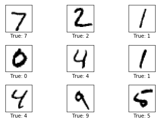
We will now create a function that is used to plot 9 images on a 3x3 grid and write the true and predicted classes under each image.
def plot_images(images, cls_true, cls_pred=None):
    assert len(images) == len(cls_true) == 9

    # Create figure with 3x3 sub-plots.
    fig, axes = plt.subplots(3, 3)
    fig.subplots_adjust(hspace=0.5, wspace=0.5)

    for i, ax in enumerate(axes.flat):
        # Plot image.
        ax.imshow(images[i].reshape(img_shape), cmap='binary')

        # Show true and predicted classes.
        if cls_pred is None:
            xlabel = "True: {0}".format(cls_true[i])
        else:
            xlabel = "True: {0}, Pred: {1}".format(cls_true[i], cls_pred[i])

        ax.set_xlabel(xlabel)

        # Remove ticks from the plot.
        ax.set_xticks([])
        ax.set_yticks([])
Let's draw some images to see if the data is correct:
# Get the first images from the test-set.
images = data.test.images[0:9]

# Get the true classes for those images.
cls_true = data.test.cls[0:9]

# Plot the images and labels using our helper-function above.
plot_images(images=images, cls_true=cls_true)
The purpose of using the TensorFlow library is to generate a computational graph that can be executed much more efficiently. TensorFlow can be more efficient than NumPy (in some cases) since TensorFlow knows the entire computation graph and its data flow that needs to be executed. NumPy on the other hand knows the computation of the math operation that is currently being executed.
TensorFlow can also automatically calculate the gradients that are needed to optimise the graph variables to make the model perform better. This is because the graph is a combination of simple mathematical expressions, so the gradient of the entire graph can be calculated using the chain rule for calculating derivatives when optimising the cost function.
A TensorFlow graph generally consists of the following parts:
Placeholder variables that are used to change the inputs (data) to the graph (links between nodes).
The variables of the model.
The model is essentially a math function that computes the results given input into the Placeholder variables and the model variables (remember that from TensorFlow's point of view, math operations are treated as graph nodes).
A measure of the cost that can be used to guide the optimisation of variables.
An optimisation method that updates the model variables.
In addition, the TensorFlow graph can also contain various debugging statements, for example to display log data using the TensorBoard, which is not covered in this tutorial.
Placeholder variables serve as input to the graph, and they can be changed as we perform operations on the graph.
Let's move on to defining the placeholder variables for the input images (Placeholder variables), which we'll call x. Doing this allows us to change the images that are fed into the TensorFlow graph.
The type of data that is introduced in the graph are vectors or multidimensional matrices (denoted tensors). These tensors are multidimensional arrays, whose form is [None, img_size_flat], where None means that the tensor can contain an arbitrary number of images, each image being a vector of length img_size_flat.
We define:
x = tf.placeholder(tf.float32, [None, img_size_flat])
Note that in the tf.placeholder function, we have to define the data type, which in this case is a float32.
Next, we define the placeholder variable for the true tags associated with the images that were entered into the x placeholder variable. The form of this placeholder variable is [None, num_classes], which means that it can hold an arbitrary number of labels, and each label is a length vector of num_classes, which is 10 in our case.
y_true = tf.placeholder(tf.float32, [None, num_classes])
Finally, we have the placeholder variable for the true class of each image in the placeholder variable x. These are integers and the dimensionality of this placeholder variable is pre-defined as [None], which means that the placeholder variable is a one-dimensional vector of arbitrary length.
y_true_cls = tf.placeholder(tf.int64, [None])
As we have indicated previously, in this example we are going to use a simple mathematical model of linear regression, that is, we are going to define a linear function where the images in the placeholder variable $x$ are multiplied by a variable w that we will call weights $y$ then add a bias that we'll call $b$.
Therefore:
\begin{equation} logist = w x + b \end{equation}
The result is a matrix of the form [num_images, num_classes], since $x$ has the form [num_images, img_size_flat] and the weight matrix $w$ has the form [img_size_flat, num_classes], so the multiplication of these two matrices is a array whose shape is [num_images, num_classes]. Then the bias vector $b$ is added to each row of that resulting matrix.
Note we have used the name $logits$ to respect typical TensorFlow terminology, but the variable can be called something else.
We define this operation in TensorFlow as follows:
zero:w = tf.Variable(tf.zeros([img_size_flat, num_classes]))
b = tf.Variable(tf.zeros([ num_classes]))
logits = tf.matmul(x, w) + b
In the definition of the $logits$ model, we have used the function tf.matmul. This function returns the value of multiplying the tensor $x$ by the tensor $w$.
The logits model is a matrix with num_images rows and num_classes columns, where the element in the i th row and j th column is an estimate of the probability that the i th input image is of the j th class.
However, these estimates are a bit difficult to interpret, since the numbers you get can be very small or very large. The next step then would be to normalise the values in such a way that, for each row of the logits matrix, all its values add up to one, thus the value of each element of the matrix is constrained between zero and one. With TensorFlow, this is calculated using the function called softmax and the result is stored in a new variable y_pred.
y_pred = tf.nn.softmax(logits)
Finally the predicted class can be computed from the y_pred array by taking the index of the largest element in each row.
y_pred_cls = tf.argmax(y_pred, dimension=1)
As we have previously indicated, the handwritten digit classification and recognition model that we have implemented is a linear regression mathematical model $logits=wx+b$. The prediction quality of the model will depend on the optimal values of the variables w (weight tensor) and b (bias tensor) given an input x (image tensor). Therefore, optimising our classifier for the digit recognition task consists of fitting our model in such a way that we can find the optimal values in the w and b tensors. This optimisation process in these variables is known as the model training or learning process.
To improve the model by classifying the input images, we must somehow find a method to change the value of the variables for the weights ($w$) and biases ($b$). To do this, we first need to know how well the model currently performs by comparing the model's predicted output y_pred to the desired output y_true. The performance function that measures the error between the actual output of the system to be modelled and the output of the estimator kernel (the model), is what is known as the cost function. Different cost functions can be defined.
Cross-entropy is a performance measure used in classification. Cross-entropy is a continuous function that is always positive and if the predicted output of the model exactly matches the desired output, then the cross entropy is equal to zero. Therefore, the goal of optimisation is to minimise the cross-entropy to get as close to zero as possible by changing the weights $w$ and biases $b$ of the model.
TensorFlow has a built-in function to calculate cross entropy. Note that the $logit$ values are used since this TensorFlow function calculates the softmax internally.
cross_entropy = tf.nn.softmax_cross_entropy_with_logits(logits=logits,labels=y_true)
Once we have calculated the cross-entropy for each of the image classifications, we have a measure of how well the model performs on each image individually. But to use cross-entropy to guide optimisation of the model variables, we need to have a single scalar value, so we simply take the average of the cross-entropy for all image classifications.
For this:
cost = tf.reduce_mean(cross_entropy)
Now that we have a cost measure to minimize, we can create an optimiser. In this case we will use one of the most used methods known as Gradient Descent (for more details see lecture 4, lecture 5 and lecture 6), where the step size for the adjustment of the variables is preset to 0.5.
Please note that optimisation is not performed at this time. In fact, nothing is calculated at all, we just add the optimiser object to the TensorFlow graph for further execution.
optimizer = tf.train.GradientDescentOptimizer(learning_rate=0.5).minimize(cost)
We need a few more performance metrics to show progress to the user. We create a vector of booleans, where we check if the predicted class is equal to the true class of each image.
correct_prediction = tf.equal(y_pred_cls, y_true_cls)
This calculates the accuracy of the classification and transforms the booleans to floats, so that False becomes 0 and True becomes 1. We then calculate the average of these numbers.
accuracy = tf.reduce_mean(tf.cast(correct_prediction, tf.float32))
Once all the elements of our model have been specified, we can now create the graph. To do this we have to create a session to then execute the graph:
session = tf.Session()
Initialise variables: Variables for weights and biases must be initialised before beginning to optimise them.
session.run(tf.global_variables_initializer())
Having 50,000 images in the training set, it can take a long time to calculate the gradient of the model using all these a images during the optimisation process. Therefore, we use a Stochastic Gradient Descent that only uses a batch of randomly selected images each iteration of the optimiser. This allows the learning process to be faster.
We create a function to perform several optimisation iterations to gradually improve the weights w and biases b of the model. At each iteration, a new batch of data is selected from the training set, and then TensorFlow runs the optimiser using those training samples. We set that batch of images to 100 (batch_size = 100).
# batch of images
batch_size = 100

def optimize(num_iterations):
    for i in range(num_iterations):
        # Get a batch of training examples.
        # x_batch now holds a batch of images and
        # y_true_batch are the true labels for those images.
        x_batch, y_true_batch = data.train.next_batch(batch_size)

        # Put the batch into a dict with the proper names
        # for placeholder variables in the TensorFlow graph.
        # Note that the placeholder for y_true_cls is not set
        # because it is not used during training.
        feed_dict_train = {x: x_batch,
                           y_true: y_true_batch}

        # Run the optimizer using this batch of training data.
        # TensorFlow assigns the variables in feed_dict_train
        # to the placeholder variables and then runs the optimizer.
        session.run(optimizer, feed_dict=feed_dict_train)
We are going to create a set of functions that will help us monitor the performance of our classifier. First we create a dictionary with the test set data that will be used as input to the TensorFlow graph.
feed_dict_test = {x: data.test.images,
                  y_true: data.test.labels,
                  y_true_cls: data.test.cls}
Function to print the classification accuracy on the test set.
def print_accuracy():
    # Use TensorFlow to compute the accuracy.
    acc = session.run(accuracy, feed_dict=feed_dict_test)

    # Print the accuracy.
    print("Accuracy on test-set: {0:.1%}".format(acc))
Function to print and plot the confusion matrix using scikit-learn.
def print_confusion_matrix():
    # Get the true classifications for the test-set.
    cls_true = data.test.cls

    # Get the predicted classifications for the test-set.
    cls_pred = session.run(y_pred_cls, feed_dict=feed_dict_test)

    # Get the confusion matrix using sklearn.
    cm = confusion_matrix(y_true=cls_true,
                          y_pred=cls_pred)

    # Print the confusion matrix as text.
    print(cm)

    # Plot the confusion matrix as an image.
    plt.imshow(cm, interpolation='nearest', cmap=plt.cm.Blues)

    # Make various adjustments to the plot.
    plt.tight_layout()
    plt.colorbar()
    tick_marks = np.arange(num_classes)
    plt.xticks(tick_marks, range(num_classes))
    plt.yticks(tick_marks, range(num_classes))
    plt.xlabel('Predicted')
    plt.ylabel('True')
Function to plot the weights of the model. 10 images are plotted, one for each digit that the model is trained to recognise.
def plot_weights():
    # Get the values for the weights from the TensorFlow variable.
    wi = session.run(w)

    # Get the lowest and highest values for the weights.
    # This is used to correct the colour intensity across
    # the images so they can be compared with each other.
    w_min = np.min(wi)
    w_max = np.max(wi)

    # Create figure with 3x4 sub-plots,
    # where the last 2 sub-plots are unused.
    fig, axes = plt.subplots(3, 4)
    fig.subplots_adjust(hspace=0.3, wspace=0.3)

    for i, ax in enumerate(axes.flat):
        # Only use the weights for the first 10 sub-plots.
        if i<10:
            # Get the weights for the i'th digit and reshape it.
            # Note that w.shape == (img_size_flat, 10)
            image = wi[:, i].reshape(img_shape)

            # Set the label for the sub-plot.
            ax.set_xlabel("Weights: {0}".format(i))

            # Plot the image.
            ax.imshow(image, vmin=w_min, vmax=w_max, cmap='seismic')

        # Remove ticks from each sub-plot.
        ax.set_xticks([])
        ax.set_yticks([])
Now that we have everything we need, let's run the classifier and do some performance testing.
Since we have already initialised the variables, the first thing we are going to look at is to see the level of precision that it has before executing any optimisation.
Let's execute the accuracy function that we have created:
print_accuracy()
Outcome:
Accuracy on test-set: 9.8%
The accuracy on the test set is 9.8%. This is because the model has only been initialised and has not been optimised at all.
We are going to use the optimisation function that we have created to an iteration:
optimize(num_iterations=1)
print_accuracy()
Outcome:
Accuracy on test-set: 40.9%
As we see after a single optimisation iteration, the model has increased its accuracy on the test set to 40.7%. This means that it misclassifies images about 6 times out of 10.
The tensor weights w can also be plotted as shown below. The positive weights take the red tones and the negative weights the blue tones. These weights can be intuitively understood as image filters.
Let's use the function plot_weights()
plot_weights()
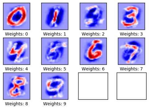
For example, the weights used to determine if an image displays a zero digit have a positive reaction (red) to the image of a circle and have a negative reaction (blue) to images with content in the center of the circle.
Similarly, the weights used to determine whether an image displays the digit 1, reacts positively (red) to a vertical line in the center of the image, and reacts negatively (blue) to images with content surrounding that line.
In these images, the weights mostly look like the digits they are supposed to recognise. This is because only one optimisation iteration has been performed, so the weights are only trained on 100 images. After training on thousands of images, the weights become more difficult to interpret because they have to recognise many variations of how the digits might be written.
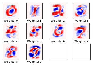
Performance after 10 iterations
# We have already performed 1 iteration.
optimize(num_iterations=9)
print_accuracy()
Outcome:
Accuracy on test-set: 78.2%
The weights
plot_weights()
Performance after 1000 optimisation iterations
# We have already performed 1000 iteration.
optimize(num_iterations=999)
print_accuracy()
plot_weights()
We obtain:
Accuracy on test-set: 92.1%
Weights
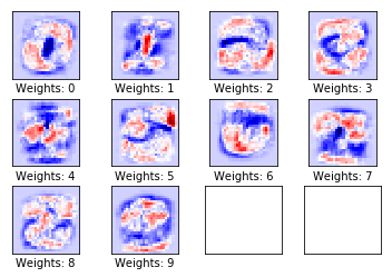
After 1,000 optimization iterations, the model only misclassifies one out of ten images. This simple model cannot achieve much better performance and therefore more complex models are needed. In subsequent tutorials, we will create a more complex model using neural networks that will help us improve the performance of our classifier.
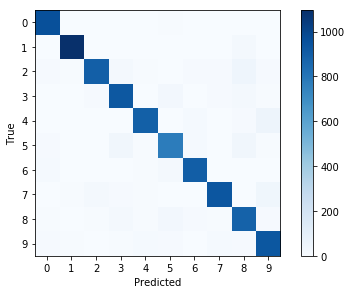
Finally, to have a global vision of the errors made by our classifier, we are going to analyse the confusion matrix.
We use our print_confusion_matrix() function.
print_confusion_matrix()
[[ 961    0    0    3    0    7    3    4    2    0]
 [   0 1097    2    4    0    2    4    2   24    0]
 [  12    8  898   23    5    4   12   12   49    9]
 [   2    0   10  927    0   28    2    9   24    8]
 [   2    1    2    2  895    0   13    4   10   53]
 [  10    1    1   37    6  774   17    4   36    6]
 [  13    3    4    2    8   19  902    3    4    0]
 [   3    6   21   12    5    1    0  936    2   42]
 [   6    3    6   18    8   26   10    5  883    9]
 [  11    5    0    7   17   11    0   16    9  933]]
Now that we're done using TensorFlow, we log out to free up its resources.
session.close()
With this we finish the first tutorial on how to use the TensorFlow library to create a linear regression model.
In the next installments we will create more complex models, including convolutional neural networks.


